Create a Relative Weights Analysis (RWA)

This function creates a Relative Weights Analysis (RWA) and returns a list of outputs. RWA provides a heuristic method for estimating the relative weight of predictor variables in multiple regression, which involves creating a multiple regression with on a set of transformed predictors which are orthogonal to each other but maximally related to the original set of predictors. rwa() is optimised for dplyr pipes and shows positive / negative signs for weights.

Usage

rwa(
  df,
  outcome,
  predictors,
  applysigns = FALSE,
  method = "auto",
  sort = TRUE,
  bootstrap = FALSE,
  n_bootstrap = 1000,
  conf_level = 0.95,
  focal = NULL,
  comprehensive = FALSE,
  include_rescaled_ci = FALSE,
  use = "pairwise.complete.obs",
  weight = NULL
)

Arguments

df

Data frame or tibble to be passed through.

outcome

Outcome variable, to be specified as a string or bare input. Must be a numeric variable.

predictors

Predictor variable(s), to be specified as a vector of string(s) or bare input(s). All variables must be numeric.

applysigns

Logical value specifying whether to show an estimate that applies the sign. Defaults to FALSE.

method

String to specify the method of regression to apply. Valid values include:

"auto": automatically detect whether to use multiple regression or logistic regression based on the outcome variable provided.
"multiple": use multiple regression.
"logistic": use logistic regression.

sort

Logical value specifying whether to sort results by rescaled relative weights in descending order. Defaults to TRUE.

bootstrap

Logical value specifying whether to calculate bootstrap confidence intervals. Defaults to FALSE. Currently only supported for multiple regression.

n_bootstrap

Number of bootstrap samples to use when bootstrap = TRUE. Defaults to 1000.

conf_level

Confidence level for bootstrap intervals. Defaults to 0.95.

focal

Focal variable for bootstrap comparisons (optional).

comprehensive

Whether to run comprehensive bootstrap analysis including random variable comparisons and, when focal is supplied, comparisons against that predictor.

include_rescaled_ci

Logical value specifying whether to include confidence intervals for rescaled weights. Defaults to FALSE due to compositional data constraints. Use with caution.

use

Method for handling missing data when computing correlations. Options are: "everything" (remaining missing values propagate, causing a non-finite correlation matrix error if correlations cannot be estimated), "all.obs" (error for remaining missing predictors in unweighted analysis), "complete.obs" (listwise deletion), "na.or.complete" (listwise deletion; no complete cases produces an insufficient-data error rather than an unusable matrix of NAs), "pairwise.complete.obs" (pairwise deletion, default). See cor for more details. Only applicable for multiple regression. Rows with missing outcomes are always removed first, including for "all.obs". When weight is specified, remaining missing weights cause an error for "all.obs" and are removed otherwise. Missing predictors are then removed by listwise deletion for every weighted mode, including "all.obs". Thus weighted correlations always use complete cases, regardless of use; weighted pairwise correlation is not implemented.

weight

Optional name of a weight variable in the data frame. If provided, a weighted correlation matrix will be computed using the specified weights. Non-missing weights must be numeric, finite, and strictly positive (zero weights are not supported). Missing weights follow the use rules. Defaults to NULL (unweighted analysis). Only applicable for multiple regression.

Value

rwa() returns a list of outputs, as follows:

predictors: character vector of names of the predictor variables used.
rsquare: the rsquare value of the regression model (multiple regression only).
result: the final output of the importance metrics (sorted by Rescaled.RelWeight in descending order by default).
- The Rescaled.RelWeight column sums up to 100.
- The Sign column indicates whether a predictor is positively or negatively correlated with the outcome.
- When bootstrap = TRUE, includes confidence interval columns for raw weights.
- When bootstrap = TRUE, Random.Diff.CI.Lower/Random.Diff.CI.Upper give the interval for the difference between each predictor's weight and the weight of a randomly generated variable, and Raw.Significant is TRUE when Random.Diff.CI.Lower is above zero. Significance is assessed this way, and not from the interval around the weight itself, because raw relative weights are non-negative: an unrelated predictor still receives a small positive weight, so an interval around it would almost always exclude zero. Comparing each weight to that of a randomly generated variable is the approach suggested by Tonidandel, LeBreton and Johnson (2009; doi:10.1037/a0017735 ) as a way to judge whether a weight exceeds what chance alone would produce. The Raw.Significant cutoff applied here is directional: a predictor is significant only when it exceeds the random variable (Random.Diff.CI.Lower > 0), because an interval lying entirely below zero indicates the predictor performed worse than noise, which is not evidence of importance in either direction.
- Rescaled weight CIs are available via include_rescaled_ci = TRUE but not recommended for inference.
n: complete-case observation count for the selected analysis variables (and weight, if supplied). Unweighted pairwise correlations may use more observations than this conservative count.
n_weighted: weighted results only; sum of original weights after all analysis filters. This is a population-size estimate only for appropriately calibrated weights and the retained population scope.
n_effective: weighted results only; Kish's unequal-weighting effective sample size, (sum(w)^2) / sum(w^2), calculated using scaled weights for numerical stability. This diagnostic ignores clustering, stratification, and weight/outcome relationships; it is not model degrees of freedom or the exact precision of RWA.
bootstrap: bootstrap results (only present when bootstrap = TRUE), containing:
- ci_results: confidence intervals for weights
- boot_object: raw bootstrap object for advanced analysis
- n_bootstrap: number of bootstrap samples used
lambda: lambda matrix from the RWA calculation.
RXX: Correlation matrix of all the predictor variables against each other. Not available for logistic regression.
RXY: Correlation values of the predictor variables against the outcome variable. Not available for logistic regression.

Details

rwa() produces raw relative weight values (epsilons) as well as rescaled weights (scaled as a percentage of predictable variance) for every predictor in the model. Signs are added to the weights when the applysigns argument is set to TRUE. See https://www.scotttonidandel.com/rwa-web for the original implementation that inspired this package.

This function is a wrapper around rwa_multiregress() and rwa_logit(), automatically selecting the appropriate method based on the outcome variable or the method argument.

In brief, for the two missing-data and weighting arguments:

Without weight, missing values are handled by use, which defaults to pairwise deletion when correlating predictors.
With weight, the analysis always uses complete cases across the outcome, the predictors, and the weight. Weighted pairwise deletion is not implemented, so use does not change a weighted result.
In both cases, rows with a missing outcome are dropped first.

Use weights when the analysis should represent a target population rather than the achieved sample. Comparing weighted with unweighted results is informative: a large difference indicates that sample composition matters.

Multiple-regression estimates require a finite joint correlation matrix. Its smallest eigenvalue must be at least minus sqrt(.Machine$double.eps) * max(1, max(abs(eigenvalues))). The predictor block must have strictly positive computed eigenvalues and the transformation must be solvable. No additional conditioning cutoff is imposed on previously estimable models; highly correlated predictors can still yield sensitive estimates. Calculated R-squared must not exceed one by more than sqrt(.Machine$double.eps); the fit is checked separately because small matrix errors can be amplified by nearly collinear predictors. An exactly fitted outcome (a singular joint matrix) is allowed when the predictor block is positive definite. Invalid matrices, constant variables, and insufficient observations cause informative errors; variables are not dropped and matrices are not silently repaired.

Weighted analysis is observation-weighted RWA. Bootstrap intervals use independent, identically distributed (iid) individual-row resampling, with each row's original weight carried along, not sampling proportional to weights. Rows with missing outcomes are removed before resampling; other missing-data filters are applied within each sample, preserving the outcome-complete sampling frame. A degenerate sample stops the bootstrap with an error: samples are not skipped, retried, or allowed to lose predictors. Clusters, strata, and replicate-weight survey designs are not supported; a weight column alone does not provide general complex-survey variance. See vignette("weighted-missing-data") for examples and limitations.

Examples

library(ggplot2)
# Basic RWA (results sorted by default)
rwa(diamonds, "price", c("depth", "carat"))
#> Parsing `price` as a non-binary variable.
#> Applying multiple regression to calculate relative weights...
#> $predictors
#> [1] "depth" "carat"
#> 
#> $rsquare
#> [1] 0.8506755
#> 
#> $result
#>   Variables Raw.RelWeight Rescaled.RelWeight Sign
#> 1     carat   0.849946308        99.91428588    +
#> 2     depth   0.000729149         0.08571412    -
#> 
#> $n
#> [1] 53940
#> 
#> $lambda
#>            [,1]       [,2]
#> [1,] 0.99990040 0.01411356
#> [2,] 0.01411356 0.99990040
#> 
#> $RXX
#>            depth      carat
#> depth 1.00000000 0.02822431
#> carat 0.02822431 1.00000000
#> 
#> $RXY
#>      depth      carat 
#> -0.0106474  0.9215913 
#> 

# RWA without sorting (preserves original predictor order)
rwa(diamonds, "price", c("depth", "carat"), sort = FALSE)
#> Parsing `price` as a non-binary variable.
#> Applying multiple regression to calculate relative weights...
#> $predictors
#> [1] "depth" "carat"
#> 
#> $rsquare
#> [1] 0.8506755
#> 
#> $result
#>   Variables Raw.RelWeight Rescaled.RelWeight Sign
#> 1     depth   0.000729149         0.08571412    -
#> 2     carat   0.849946308        99.91428588    +
#> 
#> $n
#> [1] 53940
#> 
#> $lambda
#>            [,1]       [,2]
#> [1,] 0.99990040 0.01411356
#> [2,] 0.01411356 0.99990040
#> 
#> $RXX
#>            depth      carat
#> depth 1.00000000 0.02822431
#> carat 0.02822431 1.00000000
#> 
#> $RXY
#>      depth      carat 
#> -0.0106474  0.9215913 
#> 

# Plot results using plot_rwa()
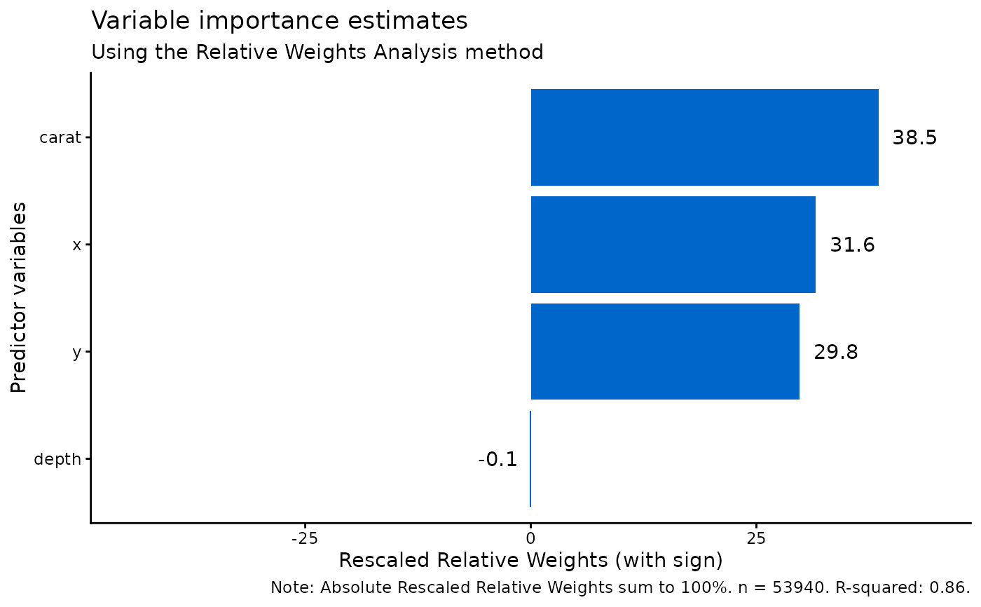
diamonds |>
  rwa("price", c("depth", "carat", "x", "y")) |>
  plot_rwa()
#> Parsing `price` as a non-binary variable.
#> Applying multiple regression to calculate relative weights...


# \donttest{
# For faster examples, use a subset of data for bootstrap
diamonds_small <- diamonds[sample(nrow(diamonds), 1000), ]

# RWA with different missing data handling
# Use complete.obs for listwise deletion
rwa(diamonds_small, "price", c("depth", "carat"), use = "complete.obs")
#> Parsing `price` as a non-binary variable.
#> Applying multiple regression to calculate relative weights...
#> $predictors
#> [1] "depth" "carat"
#> 
#> $rsquare
#> [1] 0.8506213
#> 
#> $result
#>   Variables Raw.RelWeight Rescaled.RelWeight Sign
#> 1     carat  0.8496668919         99.8878042    +
#> 2     depth  0.0009543612          0.1121958    -
#> 
#> $n
#> [1] 1000
#> 
#> $lambda
#>           [,1]      [,2]
#> [1,] 0.9999021 0.0139908
#> [2,] 0.0139908 0.9999021
#> 
#> $RXX
#>            depth      carat
#> depth 1.00000000 0.02797885
#> carat 0.02797885 1.00000000
#> 
#> $RXY
#>       depth       carat 
#> -0.01517396  0.92138091 
#> 

# RWA with weights
diamonds_small$sample_weight <- runif(nrow(diamonds_small), 0.5, 2)
rwa(diamonds_small, "price", c("depth", "carat"), weight = "sample_weight")
#> Parsing `price` as a non-binary variable.
#> Applying multiple regression to calculate relative weights...
#> $predictors
#> [1] "depth" "carat"
#> 
#> $rsquare
#> [1] 0.8538196
#> 
#> $result
#>   Variables Raw.RelWeight Rescaled.RelWeight Sign
#> 1     carat  0.8530214942        99.90652809    +
#> 2     depth  0.0007980815         0.09347191    -
#> 
#> $n
#> [1] 1000
#> 
#> $n_weighted
#> [1] 1258.593
#> 
#> $n_effective
#> [1] 895.036
#> 
#> $lambda
#>            [,1]       [,2]
#> [1,] 0.99987652 0.01571459
#> [2,] 0.01571459 0.99987652
#> 
#> $RXX
#>            depth      carat
#> depth 1.00000000 0.03142531
#> carat 0.03142531 1.00000000
#> 
#> $RXY
#>        depth        carat 
#> -0.009720205  0.923210645 
#> 

# RWA with bootstrap confidence intervals (raw weights only)
rwa(diamonds_small, "price", c("depth", "carat"),
    bootstrap = TRUE, n_bootstrap = 100)
#> Parsing `price` as a non-binary variable.
#> Applying multiple regression to calculate relative weights...
#> Running bootstrap analysis with 100 samples...
#> $predictors
#> [1] "depth" "carat"
#> 
#> $rsquare
#> [1] 0.8506213
#> 
#> $result
#>   Variables Raw.RelWeight Rescaled.RelWeight Sign Raw.RelWeight.CI.Lower
#> 1     carat  0.8496668919         99.8878042    +            0.826509375
#> 2     depth  0.0009543612          0.1121958    -           -0.001820289
#>   Raw.RelWeight.CI.Upper Random.Diff.CI.Lower Random.Diff.CI.Upper
#> 1            0.881280894          0.824920837          0.875939730
#> 2            0.001745769         -0.002465152          0.002998648
#>   Raw.Significant
#> 1            TRUE
#> 2           FALSE
#> 
#> $n
#> [1] 1000
#> 
#> $lambda
#>           [,1]      [,2]
#> [1,] 0.9999021 0.0139908
#> [2,] 0.0139908 0.9999021
#> 
#> $RXX
#>            depth      carat
#> depth 1.00000000 0.02797885
#> carat 0.02797885 1.00000000
#> 
#> $RXY
#>       depth       carat 
#> -0.01517396  0.92138091 
#> 
#> $bootstrap
#> $bootstrap$boot_object
#> 
#> ORDINARY NONPARAMETRIC BOOTSTRAP
#> 
#> 
#> Call:
#> boot::boot(data = bootstrap_data, statistic = rwa_boot_statistic, 
#>     R = n_bootstrap, outcome = outcome, predictors = predictors, 
#>     use = use, weight_var = weight)
#> 
#> 
#> Bootstrap Statistics :
#>         original        bias     std. error
#> t1* 0.0009543612  0.0003926974 0.0007904312
#> t2* 0.8496668919 -0.0005076164 0.0144265478
#> 
#> $bootstrap$boot_object_random
#> 
#> ORDINARY NONPARAMETRIC BOOTSTRAP
#> 
#> 
#> Call:
#> boot::boot(data = bootstrap_data, statistic = rwa_boot_rand_statistic, 
#>     R = n_bootstrap, outcome = outcome, predictors = predictors, 
#>     use = use, weight_var = weight)
#> 
#> 
#> Bootstrap Statistics :
#>         original       bias    std. error
#> t1* 0.0006231315 0.0002368973 0.001159848
#> t2* 0.8490193143 0.0024693300 0.013110589
#> 
#> $bootstrap$ci_results
#> $bootstrap$ci_results$raw_weights
#> # A tibble: 2 × 6
#>   variable weight_index ci_lower ci_upper ci_method ci_type
#>   <chr>           <int>    <dbl>    <dbl> <chr>     <chr>  
#> 1 depth               1 -0.00182  0.00175 basic     raw    
#> 2 carat               2  0.827    0.881   basic     raw    
#> 
#> $bootstrap$ci_results$random_comparison
#> # A tibble: 2 × 6
#>   variable weight_index ci_lower ci_upper ci_method ci_type  
#>   <chr>           <int>    <dbl>    <dbl> <chr>     <chr>    
#> 1 depth               1 -0.00247  0.00300 basic     rand_diff
#> 2 carat               2  0.825    0.876   basic     rand_diff
#> 
#> 
#> $bootstrap$n_bootstrap
#> [1] 100
#> 
#> $bootstrap$conf_level
#> [1] 0.95
#> 
#> $bootstrap$comprehensive
#> [1] FALSE
#> 
#> $bootstrap$focal
#> NULL
#> 
#> 

# Include rescaled weight CIs (use with caution for inference)
rwa(diamonds_small, "price", c("depth", "carat"),
    bootstrap = TRUE, include_rescaled_ci = TRUE, n_bootstrap = 100)
#> Parsing `price` as a non-binary variable.
#> Applying multiple regression to calculate relative weights...
#> Running bootstrap analysis with 100 samples...
#> Warning: Rescaled weight confidence intervals should be interpreted with caution due to compositional data constraints. Use for descriptive purposes only, not formal statistical inference.
#> $predictors
#> [1] "depth" "carat"
#> 
#> $rsquare
#> [1] 0.8506213
#> 
#> $result
#>   Variables Raw.RelWeight Rescaled.RelWeight Sign Raw.RelWeight.CI.Lower
#> 1     carat  0.8496668919         99.8878042    +            0.826684526
#> 2     depth  0.0009543612          0.1121958    -           -0.002100482
#>   Raw.RelWeight.CI.Upper Random.Diff.CI.Lower Random.Diff.CI.Upper
#> 1            0.882647072          0.818645103          0.879528312
#> 2            0.001687732         -0.004742914          0.001188167
#>   Raw.Significant Rescaled.RelWeight.CI.Lower Rescaled.RelWeight.CI.Upper
#> 1            TRUE                  99.7907254                 100.3545032
#> 2           FALSE                  -0.3545032                   0.2092746
#> 
#> $n
#> [1] 1000
#> 
#> $lambda
#>           [,1]      [,2]
#> [1,] 0.9999021 0.0139908
#> [2,] 0.0139908 0.9999021
#> 
#> $RXX
#>            depth      carat
#> depth 1.00000000 0.02797885
#> carat 0.02797885 1.00000000
#> 
#> $RXY
#>       depth       carat 
#> -0.01517396  0.92138091 
#> 
#> $bootstrap
#> $bootstrap$boot_object
#> 
#> ORDINARY NONPARAMETRIC BOOTSTRAP
#> 
#> 
#> Call:
#> boot::boot(data = bootstrap_data, statistic = rwa_boot_statistic, 
#>     R = n_bootstrap, outcome = outcome, predictors = predictors, 
#>     use = use, weight_var = weight)
#> 
#> 
#> Bootstrap Statistics :
#>         original        bias     std. error
#> t1* 0.0009543612  0.0004532247 0.0009073535
#> t2* 0.8496668919 -0.0005565945 0.0135365157
#> 
#> $bootstrap$boot_object_rescaled
#> 
#> ORDINARY NONPARAMETRIC BOOTSTRAP
#> 
#> 
#> Call:
#> boot::boot(data = bootstrap_data, statistic = rwa_boot_statistic_rescaled, 
#>     R = n_bootstrap, outcome = outcome, predictors = predictors, 
#>     use = use, weight_var = weight)
#> 
#> 
#> Bootstrap Statistics :
#>       original      bias    std. error
#> t1*  0.1121958  0.05395122    0.122875
#> t2* 99.8878042 -0.05395122    0.122875
#> 
#> $bootstrap$boot_object_random
#> 
#> ORDINARY NONPARAMETRIC BOOTSTRAP
#> 
#> 
#> Call:
#> boot::boot(data = bootstrap_data, statistic = rwa_boot_rand_statistic, 
#>     R = n_bootstrap, outcome = outcome, predictors = predictors, 
#>     use = use, weight_var = weight)
#> 
#> 
#> Bootstrap Statistics :
#>          original       bias    std. error
#> t1* -0.0003713048 0.0012424952 0.001138999
#> t2*  0.8470192598 0.0009944623 0.014783514
#> 
#> $bootstrap$ci_results
#> $bootstrap$ci_results$raw_weights
#> # A tibble: 2 × 6
#>   variable weight_index ci_lower ci_upper ci_method ci_type
#>   <chr>           <int>    <dbl>    <dbl> <chr>     <chr>  
#> 1 depth               1 -0.00210  0.00169 basic     raw    
#> 2 carat               2  0.827    0.883   basic     raw    
#> 
#> $bootstrap$ci_results$rescaled_weights
#> # A tibble: 2 × 6
#>   variable weight_index ci_lower ci_upper ci_method ci_type 
#>   <chr>           <int>    <dbl>    <dbl> <chr>     <chr>   
#> 1 depth               1   -0.355    0.209 basic     rescaled
#> 2 carat               2   99.8    100.    basic     rescaled
#> 
#> $bootstrap$ci_results$random_comparison
#> # A tibble: 2 × 6
#>   variable weight_index ci_lower ci_upper ci_method ci_type  
#>   <chr>           <int>    <dbl>    <dbl> <chr>     <chr>    
#> 1 depth               1 -0.00474  0.00119 basic     rand_diff
#> 2 carat               2  0.819    0.880   basic     rand_diff
#> 
#> 
#> $bootstrap$n_bootstrap
#> [1] 100
#> 
#> $bootstrap$conf_level
#> [1] 0.95
#> 
#> $bootstrap$comprehensive
#> [1] FALSE
#> 
#> $bootstrap$focal
#> NULL
#> 
#> 

# Comprehensive bootstrap analysis with focal variable
result <- rwa(diamonds_small, "price", c("depth", "carat", "table"),
              bootstrap = TRUE, comprehensive = TRUE, focal = "carat",
              n_bootstrap = 100)
#> Parsing `price` as a non-binary variable.
#> Applying multiple regression to calculate relative weights...
#> Running bootstrap analysis with 100 samples...
# View confidence intervals
result$bootstrap$ci_results
#> $raw_weights
#> # A tibble: 3 × 6
#>   variable weight_index ci_lower ci_upper ci_method ci_type
#>   <chr>           <int>    <dbl>    <dbl> <chr>     <chr>  
#> 1 depth               1 -0.00102  0.00191 basic     raw    
#> 2 carat               2  0.816    0.872   basic     raw    
#> 3 table               3 -0.00164  0.0148  basic     raw    
#> 
#> $random_comparison
#> # A tibble: 3 × 6
#>   variable weight_index ci_lower ci_upper ci_method ci_type  
#>   <chr>           <int>    <dbl>    <dbl> <chr>     <chr>    
#> 1 depth               1 -0.00193  0.00306 basic     rand_diff
#> 2 carat               2  0.814    0.879   basic     rand_diff
#> 3 table               3 -0.00252  0.0149  basic     rand_diff
#> 
#> $focal_comparison
#> # A tibble: 2 × 6
#>   variable weight_index ci_lower ci_upper ci_method ci_type   
#>   <chr>           <int>    <dbl>    <dbl> <chr>     <chr>     
#> 1 depth               1   -0.880   -0.812 basic     focal_diff
#> 2 table               2   -0.870   -0.802 basic     focal_diff
#> 
# }

# Based on logistic regression (auto-detected from binary outcome)
diamonds$IsIdeal <- as.numeric(diamonds$cut == "Ideal")
rwa(diamonds, "IsIdeal", c("depth", "carat"))
#> Parsing `IsIdeal` as a binary variable.
#> Applying logistic regression to calculate relative weights...
#> $predictors
#> [1] "depth" "carat"
#> 
#> $rsquare
#> [1] 0.02835802
#> 
#> $result
#>   Variables Raw.RelWeight Rescaled.RelWeight Sign
#> 1     carat  0.0279360368          98.511958    -
#> 2     depth  0.0004219793           1.488042    -
#> 
#> $n
#> [1] 53940
#> 
#> $lambda
#>           depth      carat
#> [1,] 0.99990040 0.01411356
#> [2,] 0.01411356 0.99990040
#>