Common Statistical Tests in R - Part I
Introduction
This post will focus on common statistical tests in R to understand and validate the relationship between two variables.
There must be tons of similar tutorials around, you may be thinking. So why?
The primary (and selfish) goal of the post is to create a guide that is practical enough for myself to refer to from time to time. This post is edited from my own notes from learning statistics and R, and have been applied to a data example/scenario that I am familiar with. This means that the examples should be easily generalisable and mostly consistent with my usual coding approach (mostly ‘tidy’ and using pipes). Along the way, this will hopefully benefit others who are learning statistics and R too.

image from Giphy
To illustrate the R code, I will be using a sample dataset
pq_data from the package vivainsights,
which is a cross-sectional time-series dataset measuring the
collaboration behaviour of simulated employees in an organization. Each
row represents an employee on a certain week, with columns measuring
behaviours such as total weekly time spent in email, meetings, chats,
and so on. The vivainsights package itself provides
visualisation and analysis functions tailored for these datasets which
are available from Microsoft
Viva Insights.
A note about the structure of this post: in the real world, one should as a best practice visually check the data distribution and run tests for assumptions like normality prior to performing any tests. For the sake of narrative and covering all the scenarios, this practice isn’t really observed in this post. Hence, please be forgiving as you see us run ‘head first’ into a test without examining the data - and avoid this in real life!
Set-up: packages and data
The package vivainsights is available on CRAN, so
you can install this with
install.packages("vivainsights").
You can load the dataset in R by calling pq_data after
loading the vivainsights package. Here is a preview of
the first ten columns of the dataset using
dplyr::glimpse():
library(vivainsights)

glimpse(pq_data[, 1:10])
## Rows: 5,593
## Columns: 10
## $ PersonId <chr> "2b625906-1f36-3273-8d0d-13e714c5f6~
## $ MetricDate <date> 2021-12-26, 2021-12-26, 2021-12-26~
## $ After_hours_call_hours <dbl> 0, 0, 0, 0, 0, 0, 0, 0, 0, 0, 0, 0,~
## $ After_hours_chat_hours <dbl> 0, 0, 0, 0, 0, 0, 0, 0, 0, 0, 0, 0,~
## $ After_hours_collaboration_hours <dbl> 7.6624994, 2.4908612, 0.1625000, 1.~
## $ After_hours_email_hours <dbl> 0.2600000, 0.5883611, 0.1625000, 0.~
## $ After_hours_meeting_hours <dbl> 7.50, 2.00, 0.00, 1.25, 19.00, 0.25~
## $ After_hours_scheduled_call_hours <dbl> 0, 0, 0, 0, 0, 0, 0, 0, 0, 0, 0, 0,~
## $ After_hours_unscheduled_call_hours <dbl> 0, 0, 0, 0, 0, 0, 0, 0, 0, 0, 0, 0,~
## $ Call_hours <dbl> 0, 0, 0, 0, 0, 0, 0, 0, 0, 0, 0, 0,~This tutorial also uses functions from tidyverse, so
ensure that you run library(tidyverse) to reproduce the
example outputs.
Framing the problem
One of the most fundamental tasks in statistics and data science is to understand the relation between two variables. Sometimes the motivation is understand whether the relationship is causal, i.e. whether one causes another. This is not always the case, as for instance, one may simply wish to test for multicollinearity when selecting predictors for a model.1
Our dataset pq_data represents the simulated
collaboration data of a company, and each row represents an employee’s
week. There are two metrics of interest:
Multitasking_hoursmeasures the total number of hours the person spent sending emails or instant messages during a meeting or a Teams call.After_hours_collaboration_hoursmeasures the number of hours a person has spent in collaboration (meetings, emails, IMs, and calls) outside of working hours.2
Imagine then we have two questions to address:
Do managers multi-task more than senior individual contributors (IC)?
The HR leadership suspects that meeting multitasking behaviour could be correlated with after-hours working, as the former represents wasted time and productivity during meetings. What can we do to understand the relationship between the two?
In this post, we will tackle the first question, and focus primarily on comparison tests and their non-parametric equivalents in R. In subsequent posts I would also like to cover other relevant tools/concepts such as correlation tests, regression tests, effect size, and statistical power.
It is worth noting that the first question postulates a relation between a categorical variable (manager/ senior IC) and a continuous variable (multitasking hours), whereas the second question a relation between two continuous variables (multitasking hours, afterhours collaboration). The types of the variables in question help determine which tests are appropriate.
The categorical variable that provides us information on whether an
employee is a manager or a senior IC in pq_data is stored
in LevelDesignation. We can use
vivainsights::hrvar_count() to explore this variable:
hrvar_count(pq_data, hrvar = "LevelDesignation")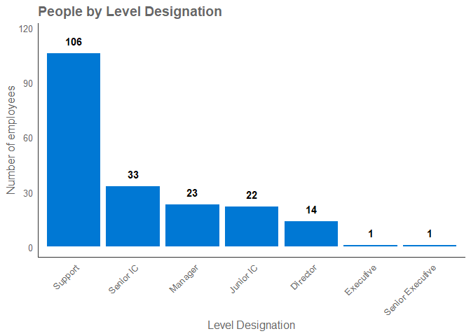
1. Comparison tests: the t-test
Two common comparison tests would be the t-test and Analysis of Variance (ANOVA). The oft-cited practical difference between the two is that you would use the t-test for comparing means between two groups, and ANOVA for more than two groups. There is a bit more nuance than that, but we will start with the t-test.
A t-test can be paired or unpaired, where the former is used for comparing the means of two groups in the same population, and the latter for independent samples from two populations or groups. Since managers and senior ICs are two different populations, an unpaired (two-sample) t-test is therefore appropriate for the scenario in question two.
Before we jump into the test, we’ll need to prepare the data. Since
we are interested in the difference between managers and senior ICs, we
will first need to create a factor variable from the data that has only
two levels. In the below code, we will first filter out any values of
LevelDesignation that are not "Manager" and
"Senior IC", and create a new factor column as
ManagerIndicator:
pq_data_grouped <-
  pq_data %>%
  filter(LevelDesignation %in% c("Manager", "Senior IC")) %>%
  mutate(
    ManagerIndicator =
      factor(LevelDesignation,
      levels = c("Manager", "Senior IC"))
  )
Recall also that our dataset pq_data is a
cross-sectional time-series dataset, which means that for every
individual identified by PersonId, there will be multiple
rows representing a snapshot of a different week. In other words, a
unique identifier would be something like a PersonWeekId.
To simplify the dataset so that we are looking at person averages, we
can group the dataset by PersonId and calculate the mean of
Multitasking_hours for each person. After this
manipulation, Multitasking_hours would represent the mean
multitasking hours per person, as opposed to per person per
week. Let us do this by building on the pipe-chain:
pq_data_grouped <-
  pq_data %>%
  filter(LevelDesignation %in% c("Manager", "Senior IC")) %>%
  mutate(
    ManagerIndicator =
      factor(LevelDesignation,
      levels = c("Manager", "Senior IC"))
  ) %>%
  group_by(PersonId, ManagerIndicator) %>%
  summarise(Multitasking_hours = mean(Multitasking_hours), .groups = "drop")

glimpse(pq_data_grouped)
## Rows: 56
## Columns: 3
## $ PersonId <chr> "00f6d464-ba1f-31ee-b51e-ab6e8ec4fb79", "023ddb61-1~
## $ ManagerIndicator <fct> Senior IC, Manager, Senior IC, Senior IC, Manager, ~
## $ Multitasking_hours <dbl> 0.2813373, 0.5980080, 0.3319752, 0.2938879, 0.70762~Now our data is in the right format.
Let us presume that the data satisfies all the assumptions of the
t-test, and see what happens when we run it with the base
t.test() function:
t.test(
  Multitasking_hours ~ ManagerIndicator,
  data = pq_data_grouped,
  paired = FALSE
)
##
## Welch Two Sample t-test
##
## data: Multitasking_hours by ManagerIndicator
## t = 10.097, df = 28.758, p-value = 5.806e-11
## alternative hypothesis: true difference in means between group Manager and group Senior IC is not equal to 0
## 95 percent confidence interval:
## 0.3444870 0.5195712
## sample estimates:
## mean in group Manager mean in group Senior IC
## 0.8103354 0.3783063In the function, the predictor and outcome variables are supplied
using a tilde (~) format common in R, and we have specified
paired = FALSE to use an unpaired t-test. As for the
output,
trepresents the t-statistic.dfrepresents the degree of freedom.p-valueis - well - the p-value. The value here shows to be significant, as it is smaller than the significance level at 0.05.- the test allows us to reject the null hypothesis that the means of multitasking hours between managers and ICs are the same.
Note that the t-test used here is the Welch’s t-test, which is an adaptation of the classic Student’s t-test. The Welch’s t-test compares the variances of the two groups (i.e. handling heteroscedasticity), whereas the classic Student’s t-test assumes the variances of the two groups to be equal (fancy term = homoscedastic).
1.1 Testing for normality
But hang on!
There are several assumptions behind the classic t-test we haven’t examined properly, namely:
- independence - sample is independent
- normality - data for each group is normally distributed
- homoscedasticity - data across samples have equal variance
We can at least be sure of (1), as we know that senior ICs and
Managers are separate populations. However, (2) and (3) are assumptions
that we have to validate and address specifically. To test whether our
data is normally distributed, we can use the Shapiro-Wilk test
of normality, with the function
shapiro.test():
pq_data_grouped %>%
  group_by(ManagerIndicator) %>%
  summarise(
    p = shapiro.test(Multitasking_hours)$p.value,
    statistic = shapiro.test(Multitasking_hours)$statistic
  )
## # A tibble: 2 x 3
## ManagerIndicator p statistic
## <fct> <dbl> <dbl>
## 1 Manager 0.146 0.936
## 2 Senior IC 0.0722 0.941As both p-values show up as less than 0.05, the test implies that we should reject the null hypothesis that the data are normally distributed (i.e. not normally distributed). To confirm, you can also perform a visual check for normality using a histogram or a Q-Q plot.
# Multitasking hours - IC
mth_ic <-
  pq_data_grouped %>%
  filter(ManagerIndicator == "Senior IC") %>%
  pull(Multitasking_hours)

qqnorm(mth_ic, pch = 1, frame = FALSE)
qqline(mth_ic, col = "steelblue", lwd = 2)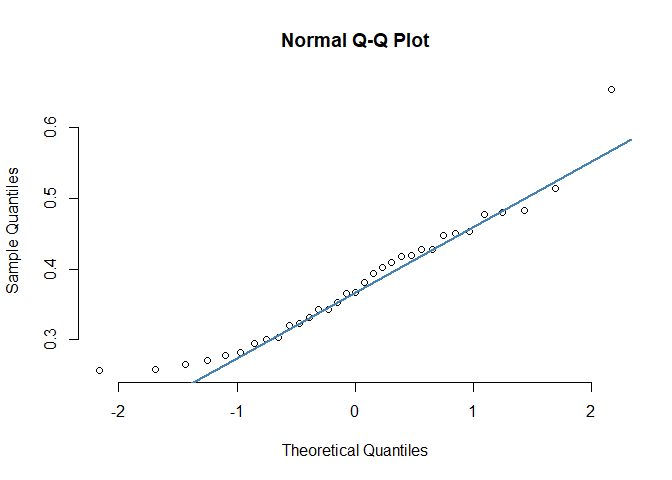
# Multitasking hours - Manager
mth_man <-
  pq_data_grouped %>%
  filter(ManagerIndicator == "Manager") %>%
  pull(Multitasking_hours)

qqnorm(mth_man, pch = 1, frame = FALSE)
qqline(mth_man, col = "steelblue", lwd = 2)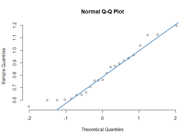
In the Q-Q plots, the points broadly adhere to the reference line. Therefore, the graphical approach suggests that the Shapiro-Wilk test may have been slightly over-sensitive. Below is a good thing to bear in mind:3
Statistical tests have the advantage of making an objective judgment of normality but have the disadvantage of sometimes not being sensitive enough at low sample sizes or overly sensitive to large sample sizes. Graphical interpretation has the advantage of allowing good judgment to assess normality in situations when numerical tests might be over or undersensitive.
In other words, the sample sizes may have well played a role in the significant result in our Shapiro-Wilk test.4 As our data isn’t conclusively normal - this in turn makes the unpaired t-test less conclusive. When we cannot safely assume normality, we can consider other alternatives such as the non-parametric two-samples Wilcoxon Rank-Sum test. This is covered further down below.
1.2 Testing for equality of variance (homoscedasticity)
Asides from normality, another assumption of the t-test that we
hadn’t properly test for prior to running t.test() is to
check for equality of variance across the two groups (homoscedasticity).
Thankfully, this was not something we had to worry about as we used the
Welch’s t-test. Recall that the classic Student’s t-test assumes
equality between the two variances, but the Welch’s t-test already takes
the difference in variance into account.
If required, however, here is an example on how you can test for
homoscedasticity in R, using var.test():
# F test to compare two variances
var.test(
  Multitasking_hours ~ ManagerIndicator,
  data = pq_data_grouped
  )
##
## F test to compare two variances
##
## data: Multitasking_hours by ManagerIndicator
## F = 4.5726, num df = 22, denom df = 32, p-value = 0.0001085
## alternative hypothesis: true ratio of variances is not equal to 1
## 95 percent confidence interval:
## 2.146082 10.318237
## sample estimates:
## ratio of variances
## 4.572575The var.test() function ran above is an F-test
(i.e. uses the F-distribution) used to compare whether the variances of
two samples are the same. Under the null hypothesis of the tests, there
should be homoscedasticity and as the f-statistic is a ratio of
variances, the f-statistic would tend towards 1. The arguments are
provided in a similar format to t.test().
It appears that homoscedasticity does not hold: since the p-value is less than 0.05, we should reject the null hypothesis that variances between the manager and IC dataset are equal. The Student’s t-test would not have been appropriate here, and we were correct to have used the Welch’s t-test.
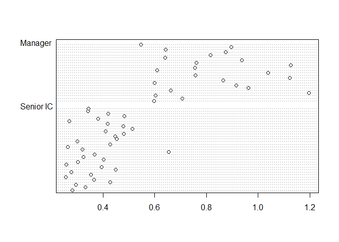
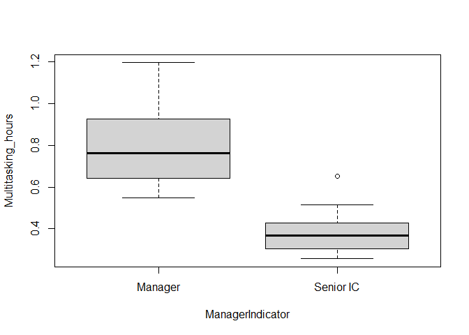
Homoscedasticity can also be examined visually, using a boxplot or a
dotplot (using graphics::dotchart() - suitable for small
datasets). The code to do so would be as follows. For this example,
visual examination is a bit more challenging as the senior IC and
Manager groups have starkly different levels of multi-tasking hours.
dotchart(
  x = pq_data_grouped$Multitasking_hours,
  groups = pq_data_grouped$ManagerIndicator
)
boxplot(
  Multitasking_hours ~ ManagerIndicator,
  data = pq_data_grouped
)
2. Non-parametric tests
2.1 Wilcoxon Rank-Sum Test
Previously, we could not safely rely on the unpaired two-sample t-test because we are not fully confident that the data satisfies the normality condition. As an alternative, we can use the Wilcoxon Rank-Sum test (aka Mann Whitney U Test). The Wilcoxon test is described as a non-parametric test, which in statistics typically means that there is no specification on a distribution, or the parameters of a distribution. In this case, the Wilcoxon test does not assume a normal distribution.
Another difference between the Wilcoxon Rank-Sum test and the unpaired t-test is that the former tests whether two populations have the same shape via comparing medians, whereas the latter parametric test compares means between two independent groups.
This is run using wilcox.test()
wilcox.test(
  Multitasking_hours ~ ManagerIndicator,
  data = pq_data_grouped,
  paired = FALSE
)
##
## Wilcoxon rank sum exact test
##
## data: Multitasking_hours by ManagerIndicator
## W = 752, p-value = 2.842e-14
## alternative hypothesis: true location shift is not equal to 0The p-value of the test is less than the significance level (alpha = 0.05), which allows us to conclude that Managers’ median multitasking hours is significantly different from the ICs’.
Note that the Wilcoxon Rank-Sum test is different from the similarly
named Wilcoxon Signed-Rank test, which is the equivalent alternative for
the paired t-test. To perform the Wilcoxon Signed-Rank test
instead, you can simply specify the argument to be
paired = TRUE. Similar to the decision of whether to use
the paired or the unpaired t-test, you should ensure that the one-sample
condition applies if you use the Wilcoxon Signed-Rank test.
2.2 Kruskal-Wallis test
So far, we have only been looking at tests which compare exactly two populations. If we are looking for a test that works with comparisons across three or more populations, we can consider the Kruskal-Wallis test.
Let us create a new data frame that is grouped at the
PersonId level, but filtering out fewer values in
LevelDesignation:
pq_data_grouped_2 <-
  pq_data %>%
  filter(LevelDesignation %in% c(
    "Support",
    "Senior IC",
    "Junior IC",
    "Manager",
    "Director"
  )) %>%
  mutate(ManagerIndicator = factor(LevelDesignation)) %>%
  group_by(PersonId, ManagerIndicator) %>%
  summarise(Multitasking_hours = mean(Multitasking_hours), .groups = "drop")

glimpse(pq_data_grouped_2)
## Rows: 198
## Columns: 3
## $ PersonId <chr> "0049ef24-ec83-356d-89f7-46b67364e677", "00f6d464-b~
## $ ManagerIndicator <fct> Support, Senior IC, Manager, Support, Support, Supp~
## $ Multitasking_hours <dbl> 0.3812649, 0.2813373, 0.5980080, 0.2918829, 0.42288~We can then run the Kruskal-Wallis test:
kruskal.test(
  Multitasking_hours ~ ManagerIndicator,
  data = pq_data_grouped_2
)
##
## Kruskal-Wallis rank sum test
##
## data: Multitasking_hours by ManagerIndicator
## Kruskal-Wallis chi-squared = 91.061, df = 4, p-value < 2.2e-16Based on the Kruskal-Wallis test, we reject the null hypothesis and
we conclude that at least one value in LevelDesignation is
different in terms of their weekly hours spent multitasking. The most
obvious downside to this method is that it does not tell us which groups
are different from which, so this may need to be followed up with
multiple pairwise-comparison tests (also known as post-hoc
tests).
3. Comparison tests: ANOVA
3.1 ANOVA
What if we want to run the t-test across more than two groups?
Analysis of Variance (ANOVA) is an alternative method that generalises the t-test beyond two groups, so it is used to compare three or more groups.
There are several versions of ANOVA. The simple version is the one-way ANOVA, but there is also two-way ANOVA which is used to estimate how the mean of a quantitative variable changes according to the levels of two categorical variables (e.g. rain/no-rain and weekend/weekday with respect to ice cream sales). In this example we will focus on one-way ANOVA.
There are three assumptions in ANOVA, and this may look familiar:
- The data are independent.
- The responses for each factor level have a normal population distribution.
- These distributions have the same variance.
These assumptions are the same as those required for the classic t-test above, and it is recommended that you check for variance and normality prior to ANOVA.
ANOVA calculates the ratio of the between-group
variance and the within-group variance
(quantified using sum of squares), and then compares this with a
threshold from the Fisher distribution (typically based on a
significance level). The key function is aov():
res_aov <-
  aov(
    Multitasking_hours ~ ManagerIndicator,
    data = pq_data_grouped_2
  )

summary(res_aov)
## Df Sum Sq Mean Sq F value Pr(>F)
## ManagerIndicator 4 40.55 10.14 504.6 <2e-16 ***
## Residuals 193 3.88 0.02
## ---
## Signif. codes: 0 '***' 0.001 '**' 0.01 '*' 0.05 '.' 0.1 ' ' 1The interpretation is as follows:5
Df: degrees of freedom for…- the outcome variable, i.e. the number of levels in the variable minus 1
- the residuals, i.e. the total number of observations minus one and minus the number of levels in the outcome variables
Sum Sq: sum of squares, i.e. the total variation between the group means and the overall meanMean Sq: mean of the sum of squares, calculated by dividing the sum of squares by the degrees of freedom for each parameterF value: test statistic from the F test. This is the mean square of each independent variable divided by the mean square of the residuals. The larger the F value, the more likely it is that the variation caused by the outcome variable is real and not due to chance.Pr(>F): p-value of the F-statistic. This shows how likely it is that the F-value calculated from the test would have occurred if the null hypothesis of no difference among group means were true.
Given that the p-value is smaller than 0.05, we reject the null
hypothesis, so we reject the hypothesis that all means are equal.
Therefore, we can conclude that at least one value in
LevelDesignation is different in terms of their weekly
hours spent multitasking.
Antoine Soetewey’s blog recommends the use of the report package, which can help you make sense of the results more easily:
library(report)

report(res_aov)
## The ANOVA (formula: Multitasking_hours ~ ManagerIndicator) suggests that:
##
## - The main effect of ManagerIndicator is statistically significant and large
## (F(4, 193) = 504.61, p < .001; Eta2 = 0.91, 95% CI [0.90, 1.00])
##
## Effect sizes were labelled following Field's (2013) recommendations.The same drawback that applies to the Kruskall-Wallis test also applies to ANOVA, in that doesn’t actually tell you which exact group is different from which; it only tells you whether any group differs significantly from the group mean. This ANOVA test is hence sometimes also referred to as an ‘omnibus’ test.
3.2 Next steps after ANOVA
A pairwise t-test (note: pairwise, not paired!) is likely required to provide more information, and it is recommended that you review the p-value adjustment methods when doing so.6 Type I errors are more likely when running t-tests pairwise across many variables, and therefore correction is necessary. Here is an example of how you might run a pairwise t-test:
pairwise.t.test(
  x = pq_data_grouped_2$Multitasking_hours,
  g = pq_data_grouped_2$ManagerIndicator,
  paired = FALSE,
  p.adjust.method = "bonferroni"
)
##
## Pairwise comparisons using t tests with pooled SD
##
## data: pq_data_grouped_2$Multitasking_hours and pq_data_grouped_2$ManagerIndicator
##
## Director Junior IC Manager Senior IC
## Junior IC <2e-16 - - -
## Manager <2e-16 <2e-16 - -
## Senior IC <2e-16 1 <2e-16 -
## Support <2e-16 1 <2e-16 1
##
## P value adjustment method: bonferroniIt may not be surprising that a pairwise method also exists as a
follow-up for the Kruskall-Wallis test - which is the pairwise Wilcoxon
test! This can be run using pairwise.wilcox.test(). The API
for the pairwise.wilcox.test() is very similar to
pairwise.t.test() where you can change the p-value
adjustment method using the argument p.adjust.method:
pairwise.wilcox.test(
  x = pq_data_grouped_2$Multitasking_hours,
  g = pq_data_grouped_2$ManagerIndicator,
  paired = FALSE,
  p.adjust.method = "bonferroni"
)
##
## Pairwise comparisons using Wilcoxon rank sum exact test
##
## data: pq_data_grouped_2$Multitasking_hours and pq_data_grouped_2$ManagerIndicator
##
## Director Junior IC Manager Senior IC
## Junior IC 5.3e-09 - - -
## Manager 3.3e-09 1.3e-09 - -
## Senior IC 5.9e-11 1 2.8e-13 -
## Support 1.3e-08 1 8.6e-13 1
##
## P value adjustment method: bonferroni4. Summary
So far, the following tests we performed have yielded similar results:
- For comparing Senior ICs and Managers:
- unpaired two-sample t-test (assumes normality)
- Wilcoxon Rank-Sum test (non-parametric)
- For comparing across more than two values:
- ANOVA (assumes normality)
- Kruskal-Wallis test (non-parametric)
- For following up on (2) with pairwise comparisons:
- pairwise t-test with correction (assumes normality)
- pairwise Wilcoxon test (non-parametric)
To the first business question, we can conclude that Senior ICs have significantly lower multitasking hours than Managers. Although the data for the two groups are not normal or equal in variance, the mitigating solutions we used have also found the differences to be significant. Moreover, it appears that significant differences also exist across other levels when we reviewed the post-hoc tests.
4.1 Should I use a t-test or ANOVA for comparing exactly two groups?
One question worth discussing is the scenario at (1). Suppose that normality is observed in both groups, does it make a difference whether I use the t-test or ANOVA if I am comparing exactly two groups?
The textbook recommendation is that whenever one is comparing exactly two groups one should use the t-test, and ANOVA whenever there are more than two groups being compared. What can get confusing here is that there is the classic Student’s t-test and the Welch’s t-test.
When ANOVA is used to compare two groups, the results will be equivalent to a classic (Student’s) t-test with equal variances.7 However, if we are talking about the Welch’s t-test instead, it may be preferable over ANOVA because the Welch’s t-test takes into account heteroscedasticity. When there is heteroscedasticity, ANOVA (as well as Kruskall-Wallis) would become unstable and produce Type I errors, such as:
- conservative estimates for large sample sizes
- inflated estimates for small sample size8
To further complicate matters, there is also a method called Welch’s
ANOVA which is like classic ANOVA but handles unequal variances better.
This can be done in R using oneway.test(), but there is
some debate around best practice that is beyond the scope of this post.
9 It
would be prudent to run the Welch versions of the tests whenever we
suspect the data to be heteroscedastic.
The recurring themes here are: (1) to check for heteroscedasticity and normality, and (2) to run multiple tests to acquire a more comprehensive view.
4.2 t-tests, ANOVA, and linear regression - are they completely different?
The common assumptions shared by the three methods may have gave it away, but the t-test, ANOVA, and linear regression are actually related in the sense that one is a special case of another.
The t-test is considered a special case of ANOVA, since the classic Student’s t-test is the same as ANOVA in comparing two groups when variances are equal. When the t-test statistic is squared, you get the corresponding f-statistic in the ANOVA.10
On the other hand, an ANOVA model is the same as a regression with a
dummy variable. In fact, the aov() function in R is a
wrapper around the linear regression function lm(). Steve
Midway’s Analysis
in R has a chapter which compares the outputs when running
ANOVA using lm() versus aov().
All of these procedures are subsumed under the General Linear Model and share the same assumptions.
End Notes
This has been a very long post - hope you have found this useful! Due to the vastness of the subject, it will not be possible to detail every consideration and method. However, this should hopefully make flow charts like the below easier to follow:
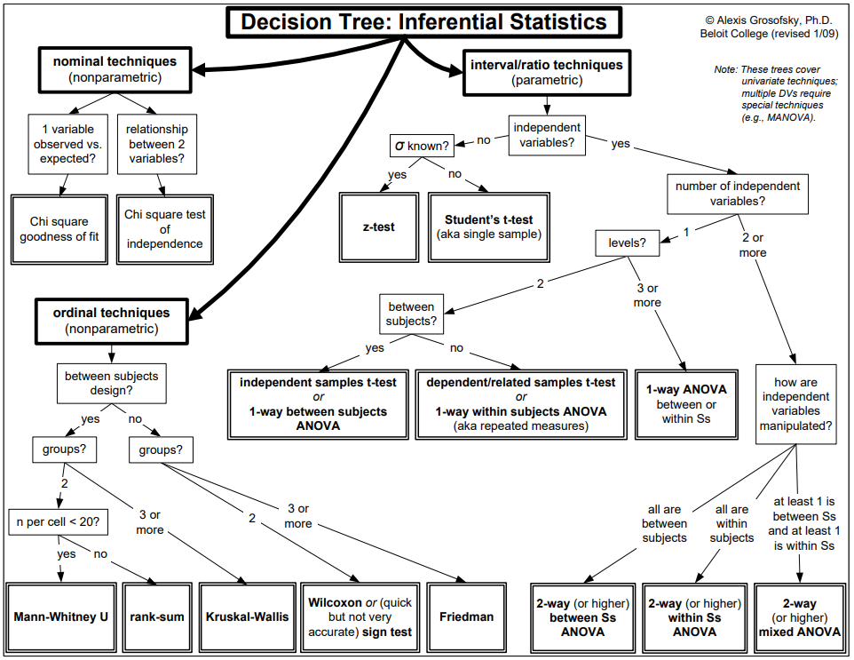
Flowchart for inferential statistics from Grosofsky (2009)
Please comment in the Disqus box down below if you have any feedback or suggestions. Do also check out the References list below for further reading; as I wrote this I have attempted to link to the brilliant resources referenced as diligently as possible.
References
a scenario in modelling where your predictor variables are correlated, which could lead to a poor inference.↩︎
See https://learn.microsoft.com/en-us/viva/insights/use/metric-definitions for definitions.↩︎
See Mishra P, Pandey CM, Singh U, Gupta A, Sahu C, Keshri A. Descriptive statistics and normality tests for statistical data. Ann Card Anaesth. 2019 Jan-Mar;22(1):67-72. doi: 10.4103/aca.ACA_157_18. PMID: 30648682; PMCID: PMC6350423.↩︎
The other well-known alternative test for normality is the Kolmogorov-Smirnoff test, run in R using
ks.test(). The KS test looks at the quantile where your empirical cumulative distribution function differs maximally from the normal’s theoretical cumulative distribution function. This is often somewhere in the middle of the distribution. On the other hand, the Shapiro-Wilk test focusses on the tails of the distribution, which is consistent to what we are seeing the Q-Q plots.↩︎References original article at https://www.scribbr.com/statistics/anova-in-r/.↩︎
An alternative is the Tukey Honest Significant Differences (
TukeyHSD()), which won’t be detailed here. TheTukeyHSD()function operates on top of the object returned byaov().↩︎See this discussion and this.↩︎
See https://statisticsbyjim.com/anova/welchs-anova-compared-to-classic-one-way-anova/; https://blog.minitab.com/en/adventures-in-statistics-2/did-welchs-anova-make-fishers-classic-one-way-anova-obsolete; http://ritsokiguess.site/docs/2017/05/19/welch-analysis-of-variance/. See also Liu, H. (2015). Comparing Welch ANOVA, a Kruskal-Wallis test, and traditional ANOVA in case of heterogeneity of variance. Virginia Commonwealth University.↩︎
It is worth a quick footnote on the differences between the t-statistic and the f-statistic. The f-statistic is an output that is found in both the F-tests for variance (see
var.test()) and ANOVA (seeaov()). The f-statistic is a ratio of two variances, and variance is squared standard deviation. Note that the f-tests for variance and ANOVA are not the same, as the former compares variances of two populations whereas the latter compares within- and between-group variances, even though both tests use the f-distribution. When there are only two groups for the one-way ANOVA F-test, the f-statistic is equal to the square of the Student’s t-statistic.↩︎
