
Vignette: Google Trends with the gtrendsR package
Background
Google Trends is a well-known, free tool provided by Google that allows you to analyse the popularity of top search queries on its Google search engine. In market exploration work, we often use Google Trends to get a very quick view of what behaviours, language, and general things are trending in a market.
And of course, if you can do something in R, then why not do it in R?
Philippe Massicotte’s gtrendsR is pretty much the go-to package for running Google Trends queries in R. It’s simple, you don’t need to set up API keys or anything, and it’s fairly intuitive. Let’s have a go at this with a simple and recent example.
Example: A Controversial Song from Hong Kong

Glory to Hong Kong (Chinese: 願榮光歸香港) is a Cantonese march song which became highly controversial politically, due to its wide adoption as the “anthem” of the Hong Kong protests. Since it was written collaboratively by netizens in August 2019,1 the piece has become viral and was performed all over the world and translated into many different languages.2 It’s also available on Spotify - just to give you a bit of context of its popularity.
Analytically, it would be interesting to compare the Google search trends of the English search term (“Glory to Hong Kong”) and the Chinese search term (“願榮光歸香港”), and see what they yield respectively. When did it go viral, and which search term is more popular? Let’s find out.
Using gtrendsR
gtrendsR is available on CRAN, so just make sure it’s installed (install.packages("gtrendsR")) and load it. Let’s load tidyverse as well, which we’ll need for the basic data cleaning and plotting:
library(gtrendsR)
library(tidyverse)
The next step then is to assign our search terms to a character variable called search_terms, and then use the package’s main function gtrends().
Let’s set the geo argument to Hong Kong only, and limit the search period to 12 months prior to today. We’ll assign the output to a variable - and let’s call it output_results.
search_terms <- c("Glory to Hong Kong", "願榮光歸香港")

gtrends(keyword = search_terms,
        geo = "HK",
        time = "today 12-m") -> output_results
output_results is a gtrends/list object, which you can extract all kinds of data from:
##                     Length Class      Mode
## interest_over_time  7      data.frame list
## interest_by_country 0      -none-     NULL
## interest_by_region  0      -none-     NULL
## interest_by_dma     0      -none-     NULL
## interest_by_city    0      -none-     NULL
## related_topics      0      -none-     NULL
## related_queries     6      data.frame list
Let’s have a look at interest_over_time, which is primarily what we’re interested in. You can access the data frame with the $ operator, and check out the data structure:
output_results %>%
  .$interest_over_time %>%
  glimpse()
## Observations: 104
## Variables: 7
## $ date <dttm> 2018-10-21, 2018-10-28, 2018-11-04, 2018-11-11, 2018...
## $ hits <int> 0, 0, 0, 0, 0, 0, 0, 0, 0, 0, 0, 0, 0, 0, 0, 0, 0, 0,...
## $ geo <chr> "HK", "HK", "HK", "HK", "HK", "HK", "HK", "HK", "HK",...
## $ time <chr> "today 12-m", "today 12-m", "today 12-m", "today 12-m...
## $ keyword <chr> "Glory to Hong Kong", "Glory to Hong Kong", "Glory to...
## $ gprop <chr> "web", "web", "web", "web", "web", "web", "web", "web...
## $ category <int> 0, 0, 0, 0, 0, 0, 0, 0, 0, 0, 0, 0, 0, 0, 0, 0, 0, 0,...This is what the hits variable represents, according to Google’s FAQ documentation:
Google Trends normalizes search data to make comparisons between terms easier. Search results are normalized to the time and location of a query by the following process:
Each data point is divided by the total searches of the geography and time range it represents to compare relative popularity. Otherwise, places with the most search volume would always be ranked highest.
The resulting numbers are then scaled on a range of 0 to 100 based on a topic’s proportion to all searches on all topics.
Let us plot this in ggplot2, just to try and replicate what we normally see on the Google Trends site - i.e. visualising the search trends over time. I really like the Economist theme from ggthemes, so I’ll use that:
output_results %>%
  .$interest_over_time %>%
  ggplot(aes(x = date, y = hits)) +
  geom_line(colour = "darkblue", size = 1.5) +
  facet_wrap(~keyword) +
  ggthemes::theme_economist() -> plot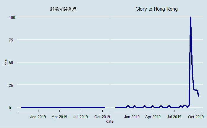
This finding above is surprising, because you would expect that Hong Kong people are more likely to search for the Chinese term rather than the English term, as the original piece was written in Cantonese.
I’ll now re-run this piece of analysis, using the shorter term 榮光, as the hypothesis is that people are more likely to search for that instead of the full song name. It could also be a quirk of Google Trends that it doesn’t return long Chinese search queries properly.
I’ll try to do this in a single pipe-line. Note what’s done differently this time:
timeis set to 3 months from today- The
onlyInterestargument is set toTRUE, which only returns interest over time and therefore is faster. - Google Trends returns hits as <1 as a character value for a value lower than 1, so let’s replace that with an arbitrary value 0.5 so we can plot this properly (the
hitsvariable needs to be numeric).
gtrends(keyword = c("Glory to Hong Kong", "榮光"),
        geo = "HK",
        time = "today 3-m",
        onlyInterest = TRUE) %>%
  .$interest_over_time %>%
  mutate_at("hits", ~ifelse(. == "<1", 0.5, .)) %>% # replace with 0.5
  mutate_at("hits", ~as.numeric(.)) %>% # convert to numeric
  # Begin ggplot
  ggplot(aes(x = date, y = hits)) +
  geom_line(colour = "darkblue", size = 1.5) +
  facet_wrap(~keyword) +
  ggthemes::theme_economist() -> plot2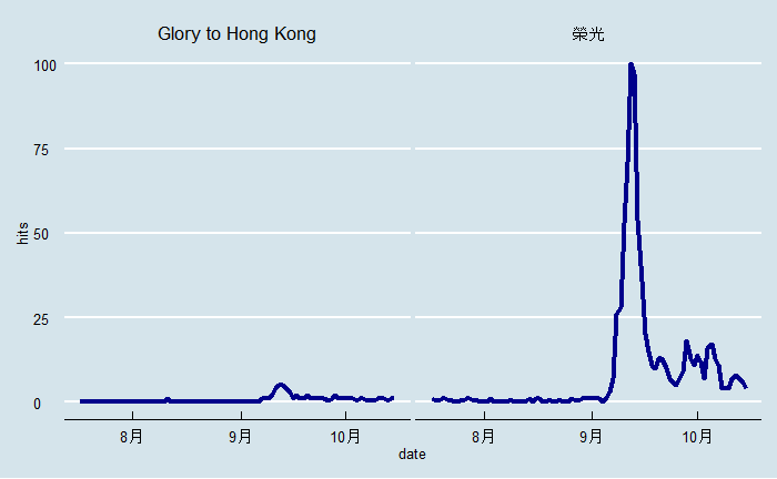
There you go! This is a much more intuitive result, where you’ll find that the search term for “榮光” reaches its peak in mid-September of 2019, whereas search volume for the English term is relatively lower, but still peaks at the same time.
I should caveat that the term “榮光” simply means Glory in Chinese, which people could search for without necessarily searching for the song, but we can be pretty sure that in the context of what’s happening that this search term relates to the actual song itself.
Limitations
One major limitation of Google Trends is that you can only search a maximum of five terms at the same time, which means that there isn’t really a way to do this at scale. There are some attempts online of doing multiple searches and “connect” the searches together by calculating an index, but so far I’ve not come across any attempts which have yielded a very satisfactory result. However, this is more of a limitation of Google Trends than the package itself.
What you can ultimately do with the gtrendsR package is limited by what Google provides, but the benefit of using gtrendsR is that all your search inputs will be documented, and certainly helps towards a reproducible workflow.
End notes / side discussion
This might just be another one of those things you can do in R, but the benefit is relatively minimal given that you cannot scale it very much. This reminds me of a meme:

Still, I suppose you can do a lot worse.
Also, writing this particular post made me realise how much more faff is involved when your post features a non-English language and you have to make changes to the encoding - Jekyll (the engine used for generating the static HTML pages on GitHub) isn’t particularly friendly for this purpose. Might be a subject for a separate discussion!
https://en.wikipedia.org/wiki/Glory_to_Hong_Kong. For more information about the Hong Kong protests, check out https://www.helphk.info/.↩