
Working with SPSS labels in R
TL;DR 📖
This post provides an overview of R functions for dealing with survey data labels, particularly ones that I wish I’d known when I first started out analysing survey data in R. Some of these functions come from surveytoolbox, a package I’m developing (GitHub only) which contains a collection of my favourite / most frequently used R functions for analysing survey data. I also highly recommend checking out labelled, sjlabelled, and of course tidyverse’s own haven package 📦.

Background
Since a significant proportion of my typical analysis projects involves survey data, I’m always on the look out for new and better ways to improve my R analysis workflows for surveys. Funnily enough, when I first started out to use R a couple of years ago, I didn’t think R was at all intuitive or easy to work with survey data. Rather painful if I’m completely honest!
One of the big reasons for this “pain” was due to survey labels.1
Survey data generally cannot be analysed independently of the variable labels (e.g. Q1. What is your gender?) and value labels (e.g. 1 = Male, 2 = Female, 3 = Other, …), which is true in the case of categorical variables.
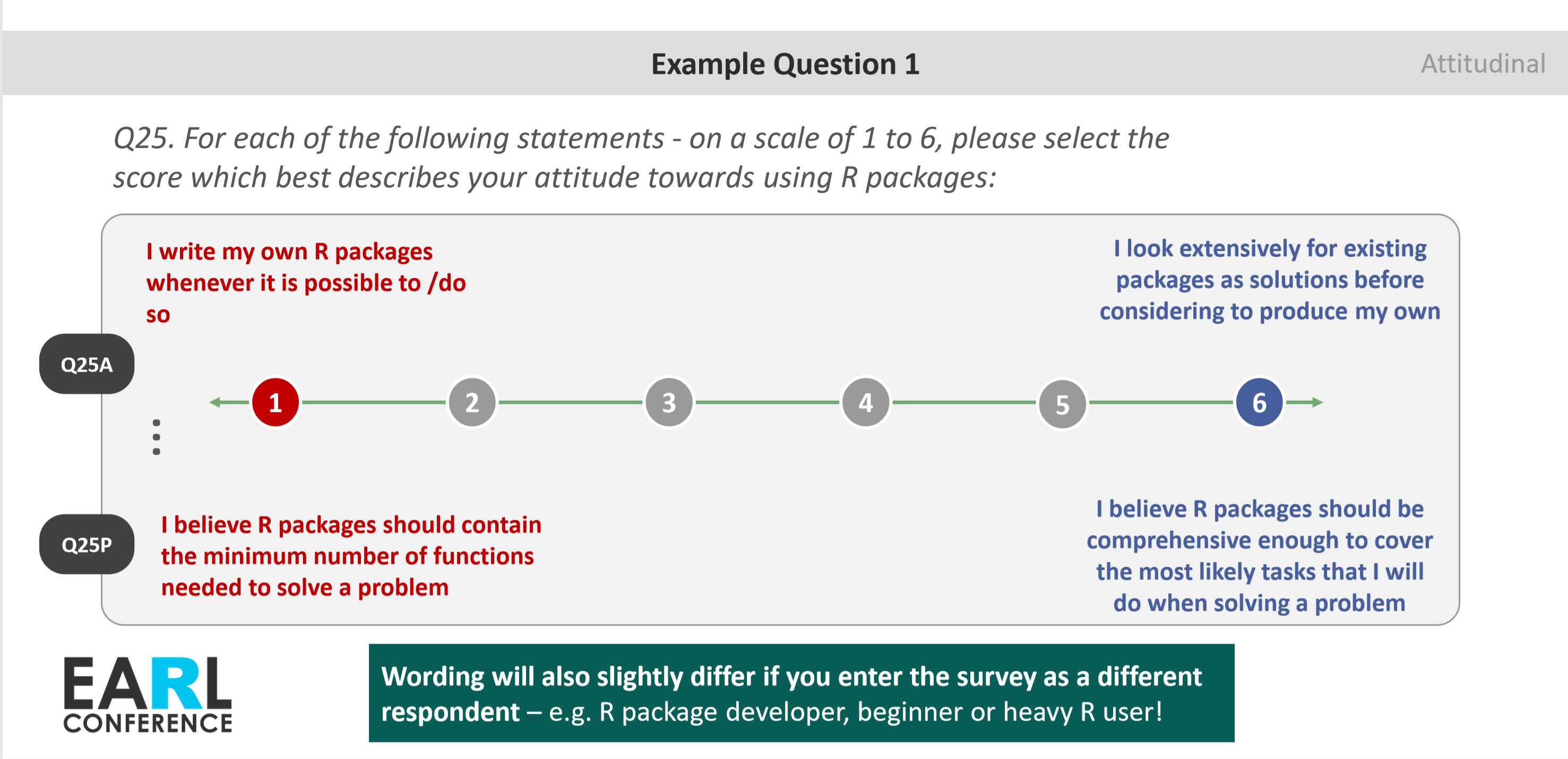
Even for ordinal Likert scale variables such as “On a scale of 1 to 10, how much do you agree with…”, the meaning of the value is highly dependent on the nuanced wording of the agree-disagree statement. For instance:
- Respondents with a different classification within the survey (e.g. “full-time employees” vs “retirees”) may also have answered a statement that is worded slightly differently but their responses are reflected using a single variable in the data: for instance, employees may be asked about their satisfaction with their current employer in the survey, and retirees asked about their previous employer.
- In my talk at the EARL conference last year, I also discussed a specific type of trade-off agreement question where any interpretation of the data is particularly sensitive to the value labels:
My experience was that the base data frame in R does not easily lend itself to work easily with these labels. A lot of merging, sorting, recoding etc. therefore is then necessary in order to turn the analysis into neat output contingency tables that you typically get via other specialist survey analysis software, like SPSS or Q. Here’s an example (with completely made up numbers) of what I would typically need to produce as an output:
## # A tibble: 3 x 3
##   `Q10 Top 2 Box Agree`                 `R Users Segmen~ `Python Users Seg~
##   <chr>                                 <chr>            <chr>
## 1 Coding R is one of my hobbies         88.1%            60.0%
## 2 I don't like to spend time in front ~ 40.5%            39.1%
## 3 I would be inclined to quit my job i~ 70.1%            40.5%
Of course, another big reason was my own ignorance of all the different methods and packages available out there at the time, which would have otherwise made a lot of this easier! 😛
This post provides a tour of the various functions (from different packages) that I wish I had known at the time. Despite the title, it’s not just about SPSS: there are plenty of other formats (e.g. SAS files) out there which carry variable and value labels, but I think this title is justified because:
- Most people starting out on survey data analysis will tend to first come across SPSS files (.sav)
- SPSS is still one of the most popular data formats for survey data
- It’s a SPSS file that I will use as a demo in this post - and the importing functions which I will briefly go through are SPSS-specific
Let’s start! 🚀
Let us first load in all the packages that we’ll use in this post. For clarity, I will still make the package-source of the functions explicit (e.g. labelled::val_label()) so it’s easy to see where each function comes from. One of these packages surveytoolbox is my own and available on Github only, and if you’re interested you can install this by running devtools::install_github("martinctc/surveytoolbox").
library(tidyverse)
library(haven)
library(sjlabelled)
library(labelled)
library(surveytoolbox) # install with devtools::install_github("martinctc/surveytoolbox")
Since all I really needed is just an open-source, simple, and accessible SPSS / .sav dataset with variable and value labels that I could use for examples, I simply went online and found the first dataset that ticked these boxes. Not the most exciting - it’s the 1991 General Social Survey, which is a nationally representative sample of adults in the United States. You can download the SAV file from the ARDA site here.
haven::read_sav() is my favourite way of loading in SPSS files. In my experience, it rarely has any problems and is generally fast enough; it is also part of the tidyverse. There are other alternatives such as sjlabelled::read_spss() and foreign::read.spss(), but haven is my personal recommendation - you can pick a favourite and have these available in your backpocket.2 Two points to note:
foreign::read.spss()returns a list rather than a data frame or a tibble, which for me is less ideal for analysis.Another method for importing SPSS files is rio’s
import()function. I understand that this is just a wrapper around haven’sread_sav()function, so I won’t discuss this method here.
Let’s load in the same SPSS file, using the different methods:
file_path <- "../datasets/General Social Survey_1991.SAV"

source_data_hv <- haven::read_sav(file_path)
source_data_sj <- sjlabelled::read_spss(file_path)
source_data_fo <- foreign::read.spss(file_path)
Running glimpse() on the first twenty rows of the imported data show that many variables are of the labelled double class (where it shows <dbl+lbl>) - meaning that these variables would have labels associated with the numeric values they hold. The numeric values alone us tell us nothing about what they represent, as these are likely to be categorical variables “in reality”.
source_data_hv %>% # File read in using `haven::read_sav()`
  .[,1:20] %>% # First 20 columns
  glimpse()
## Observations: 1,517
## Variables: 20
## $ YEAR <dbl+lbl> 1991, 1991, 1991, 1991, 1991, 1991, 1991, 1991, 1...
## $ ID <dbl> 1, 2, 3, 4, 5, 6, 7, 8, 9, 10, 11, 12, 13, 14, 15, 16...
## $ WRKSTAT <dbl+lbl> 1, 2, 1, 1, 2, 8, 1, 6, 7, 1, 1, 7, 1, 1, 1, 7, 1...
## $ HRS1 <dbl+lbl> 40, 20, 50, 45, 20, NA, 40, NA, NA, 30, 40, NA, 4...
## $ HRS2 <dbl> NA, NA, NA, NA, NA, NA, NA, NA, NA, NA, NA, NA, NA, N...
## $ EVWORK <dbl+lbl> NA, NA, NA, NA, NA, 2, NA, 1, 2, NA, NA, 1, NA, N...
## $ WRKSLF <dbl+lbl> 2, 2, 2, 2, 2, NA, 1, 2, NA, 2, 2, 2, 2, 2, 2, NA...
## $ OCC80 <dbl> 453, 178, 7, 197, 447, NA, 999, 207, NA, 803, 723, 74...
## $ PRESTG80 <dbl> 22, 75, 59, 48, 42, NA, NA, 60, NA, 38, 36, 28, 65, 4...
## $ INDUS80 <dbl> 772, 841, 700, 800, 731, NA, 999, 832, NA, 632, 342, ...
## $ MARITAL <dbl+lbl> 3, 1, 1, 5, 5, 5, 5, 4, 3, 1, 5, 1, 1, 5, 4, 1, 3...
## $ AGEWED <dbl+lbl> 20, 24, 33, NA, NA, NA, NA, 21, 19, 25, NA, 23, 2...
## $ DIVORCE <dbl+lbl> NA, 2, 2, NA, NA, NA, NA, NA, NA, 2, NA, 2, 2, NA...
## $ WIDOWED <dbl+lbl> 2, 2, 2, NA, NA, NA, NA, 2, 2, 2, NA, 1, 2, NA, 2...
## $ SPWRKSTA <dbl+lbl> NA, 1, 7, NA, NA, NA, NA, NA, NA, 1, NA, 5, 1, NA...
## $ SPHRS1 <dbl+lbl> NA, 40, NA, NA, NA, NA, NA, NA, NA, 35, NA, NA, 4...
## $ SPHRS2 <dbl+lbl> NA, NA, NA, NA, NA, NA, NA, NA, NA, NA, NA, NA, N...
## $ SPEVWORK <dbl+lbl> NA, NA, 1, NA, NA, NA, NA, NA, NA, NA, NA, 1, NA,...
## $ SPWRKSLF <dbl+lbl> NA, 1, 2, NA, NA, NA, NA, NA, NA, 2, NA, 2, 2, NA...
## $ SPOCC80 <dbl> NA, 13, 7, NA, NA, NA, NA, NA, NA, 6, NA, 417, 19, NA...Note that haven::read_sav() reads these labelled variables in as a class called haven_labelled, whilst sjlabelled::read_spss() would read these in as numeric variables containing label attributes. You can check this by running class() on one of the labelled variables.
Using haven:
## [1] "haven_labelled"Using sjlabelled:
## [1] "numeric"Running attr() whilst specifying “labels” shows that both methods of reading the SPSS file return variables that contain value label attributes. Note that specifying “labels” (with an s) typically returns value labels, whereas “label” (no s) would return the variable labels.
Viewing value labels for data imported using haven:
##       Married       Widowed      Divorced     Separated Never married
##             1             2             3             4             5
Viewing value labels for data imported using sjlabelled:
##       Married       Widowed      Divorced     Separated Never married
##             1             2             3             4             5
Viewing variable labels for data imported using haven:
## [1] "Are you currently -- married, widowed, divorced, separated, or have you never been married?"Viewing variable labels for data imported using sjlabelled:
## [1] "Are you currently -- married, widowed, divorced, separated, or have you never been married?"As you can see, there are no differences in the labels returned whether the data is imported using haven or sjlabelled.
It’s also worth noting that various different packages have similar methods for extracting variable and value labels - which practically do the same thing:
list(
  "labelled::var_label()" = source_data_sj$MARITAL %>% labelled::var_label(),
  "sjlabelled::get_label()" = source_data_sj$MARITAL %>% sjlabelled::get_label(),
  "attr()" = source_data_sj$MARITAL %>% attr(which = "label")
)
## $`labelled::var_label()`
## [1] "Are you currently -- married, widowed, divorced, separated, or have you never been married?"
##
## $`sjlabelled::get_label()`
## [1] "Are you currently -- married, widowed, divorced, separated, or have you never been married?"
##
## $`attr()`
## [1] "Are you currently -- married, widowed, divorced, separated, or have you never been married?"Exploring labels in the dataset 🔎
For the subsequent examples, I’ll only reference the tibble returned with haven::read_sav() for simplicity.
Before you perform any analysis, it’s necessary to first explore what variables and variable codes (value labels) are available in the data, which is needed if you do not have the original questionnaire. Here are several of my favourite functions:
sjPlot::view_df()surveytoolbox::varl_tb()surveytoolbox::extract_vallab()labelled::look_for()
sjPlot::view_df()
The view_df() function from the sjPlot package returns a pretty HTML document that, by default, contains a table that details the following for all the variables in the data:
- Variable name
- Variable label
- Value range / Values
- Value labels
Here’s a screenshot of the generated document: 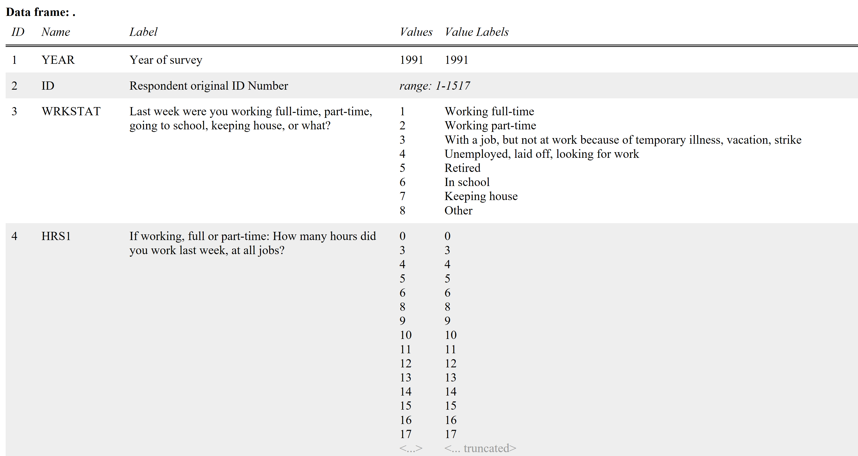
Check out this link to see a full example of what’s generated with the function:
The documentation for view_df() also states that you can show percentages and frequencies for each variable, which is a pretty nifty feature for exploring a dataset.
surveytoolbox::varl_tb()
But what if you wished to extract individual labels for further formatting / analysis?
The varl_tb() from the surveytoolbox allows you to export variable names and their labels, returning a tidy data frame. This provides a convenient way of extracting labels if there is a desire to run string manipulation operations on the labels to be used for something else. This is what the output looks like if you run varl_tb() on the first twenty columns of our dataset:
## NOT RUN - USE THIS TO INSTALL THE surveytoolbox PACKAGE
# devtools::install_github("martinctc/surveytoolbox")

source_data_hv %>%
  .[,1:20] %>%
  varl_tb()
## # A tibble: 20 x 2
## var var_label
## <chr> <chr>
## 1 YEAR Year of survey
## 2 ID Respondent original ID Number
## 3 WRKSTAT Last week were you working full-time, part-time, going to scho~
## 4 HRS1 If working, full or part-time: How many hours did you work las~
## 5 HRS2 If with a job, but not at work: How many hours a week do you u~
## 6 EVWORK If retired, in school, keeping house, or other: Did you ever w~
## 7 WRKSLF (Are/Were) you self-employed or (do/did) you work for someone ~
## 8 OCC80 Respondent's occupation (See Note 1: Occupational Codes and Pr~
## 9 PRESTG80 Prestige of respondent's occupation (See Note 1: Occupational ~
## 10 INDUS80 Respondent's industry (See Note 2: Industrial Classification o~
## 11 MARITAL Are you currently -- married, widowed, divorced, separated, or~
## 12 AGEWED If ever married: How old were you when you first married?
## 13 DIVORCE If currently married or widowed: Have you ever been divorced o~
## 14 WIDOWED If currently married, separated, or divorced: Have you ever be~
## 15 SPWRKSTA Last week was your (wife/husband) working full-time, part-time~
## 16 SPHRS1 If working, full or part-time: How many hours did (he/she) wor~
## 17 SPHRS2 If with a job, but not at work: How many hours a week does (he~
## 18 SPEVWORK If spouse retired, in school, keeping house, or other: Did (he~
## 19 SPWRKSLF (Is/Was) (he/she) self-employed or (does/did) (he/she) work fo~
## 20 SPOCC80 Respondent's spouse's occupation (See Note 1: Occupational Cod~The additional benefit of this function is that this is all magrittr-pipe optimised, so this fits perfectly with a dplyr-oriented workflow.
surveytoolbox::extract_vallab()
If you’re interested in extracting individual value labels, another method is available within surveytoolbox through extract_vallab(). This is easy: simply enter the variable name as the second argument (as a string):
## # A tibble: 8 x 2
##      id WRKSTAT
##   <dbl> <chr>
## 1     1 Working full-time
## 2     2 Working part-time
## 3     3 With a job, but not at work because of temporary illness, vacation~
## 4     4 Unemployed, laid off, looking for work
## 5     5 Retired
## 6     6 In school
## 7     7 Keeping house
## 8     8 Other
You can then use the output from extract_vallab() for joining / editing labels with analysis outputs if needed.
labelled::look_for()
But what if you’re not sure about the exact variable names, but you know roughly what’s in the variable label (typically, survey question text)? labelled::look_for() provides a pipe-optimised method that allows you to search into both variable names and variable label descriptions. Say for instance we want to identify a variable relating to household income deficit, where “income deficit” are the keywords. The look_for() function then returns a data frame with a “variable” column and a “label” column:
##     variable                       label
## 644   INCDEF Income deficit of household
You can then very easily browse the value labels of INCDEF with surveytoolbox::extract_vallab():
## # A tibble: 8 x 2
##      id INCDEF
##   <dbl> <chr>
## 1     1 -$10,000
## 2     2 -$10,000 to -$5,000
## 3     3 -$4,999 to -$1,000
## 4     4 -$999 to +$999
## 5     5 +$1,000 to $4,999
## 6     6 +$5,000 to +$10,000
## 7     7 +$10,000
## 8     8 $20,000 +
To be continued..!
Working with survey data labels is itself a pretty big subject (surprisingly), and this post has only very much just scraped the surface. For instance, factors is another subject that deserves exploration, as they are the standard R class for working with categorical data. A quick Google search will reveal more packages that allow you to deal with labels, such as expss, which I haven’t used before. It’s typically a valuable exercise anyway to compare and benchmark different methods on consistency, versatility, and speed - as this will inform you on which method will likely work best for your workflow. Therefore there will (probably) be a part 2 to this post!
The good and bad thing about R is there are often many ways to do a similar thing (see this discussion), and therefore it’s often useful to compare and contrast functions from different packages that do similar things. The functions discussed in this post is what I’ve personally found to work well with my own workflow / code, and by no means is this an exhaustive, comprehensive survey of methods!
I very much would like to hear any comments / feedback that you have with either the content on this blog or with the surveytoolbox package. Thank you!
If you’ve got some spare time, please have a read of this additional footnote 3 on why it took me slightly longer to publish this post.
In this post, the focus of the dicussion would be more on labelled vectors than factors; in line with the principle listed in haven’s documentation on the labelled function, the best practice is to analyse the data using a standard R class, but knowing how to deal with labels is useful at the importing / data checking stage.↩
See this blog post for a more in-depth discussion on the differences↩
I had planned to finish this post earlier in the week, but distressing news from my home city Hong Kong has diverted my attention. In the past week, a million Hong Kongers had been peacefully protesting against a bill which will enable extradition to mainland China, which has a record of questionable judicial processes. In the last 1-2 days, this peaceful process has turned violent with the government first declaring the protest as a ‘riot’ based on a small minority of resistance, then with the police injuring defenseless citizens with rubber bullet and tear gas rounds, with students and people I know amongst the victims. I want to express support for those are still peacefully resisting on the streets as I write, and to hopefully raise awareness of what is happening in Hong Kong to everyone around the world. Please check out this explainer by the Guardian to find out more.↩